MATHEMATICIAN-
(1)Christian Felix Klein (25 April 1849 – 22 June 1925) was a German mathematician and mathematics educator, known for his work in group theory, complex analysis, non-Euclidean geometry, and on the connections between geometry and group theory. His 1872 Erlangen Program, classifying geometries by their underlying symmetry groups, was a hugely influential synthesis of much of the mathematics of the day.
-HIS WORK- 
Klein's dissertation, on line geometry and its applications to mechanics, classified second degree line complexes using Weierstrass's theory of elementary divisors.
Klein's first important mathematical discoveries were made in 1870. In collaboration with Sophus Lie, he discovered the fundamental properties of the asymptotic lines on the Kummer surface. They went on to investigate W-curves, curves invariant under a group of projective transformations. It was Lie who introduced Klein to the concept of group, which was to play a major role in his later work. Klein also learned about groups from Camille Jordan.^[11]

A hand-blown Klein Bottle

Klein devised the bottle named after him, a one-sided closed surface which cannot be embedded in three-dimensional Euclidean space, but it may be immersed as a cylinder looped back through itself to join with its other end from the "inside". It may be embedded in Euclidean space of dimensions 4 and higher.
In the 1890s, Klein turned to mathematical physics, a subject from which he had never strayed far, writing on the gyroscope with Arnold Sommerfeld.^[12] In 1894 he launched the idea of an encyclopedia of mathematics including its applications, which became the Enzyklopädie der mathematischen Wissenschaften. This enterprise, which ran until 1935, provided an important standard reference of enduring value.^[13]

(2)Stefan Banach ([ˈstɛfan ˈbanax]  30 March 1892 – 31 August 1945) was a Polish mathematician who is generally considered one of the world's most important and influential 20th-century mathematicians. He was one of the founders of modern functional analysis, and an original member of the Lwów School of Mathematics. His major work was the 1932 book, Théorie des opérations linéaires (Theory of Linear Operations), the first monograph on the general theory of functional analysis.

Banach's dissertation, completed in 1920 and published in 1922, formally axiomatized the concept of a complete normed vector space and laid the foundations for the area of functional analysis. In this work Banach called such spaces "class E-spaces", but in his 1932 book, Théorie des opérations linéaires, he changed terminology and referred to them as "spaces of type B", which most likely contributed to the subsequent eponymous naming of these spaces after him.^[20] The theory of what came to be known as Banach spaces had antecedents in the work of the Hungarian mathematician Frigyes Riesz (published in 1916) and contemporaneous contributions from Hans Hahn and Norbert Wiener.^[14] For a brief period in fact, complete normed linear spaces were referred to as "Banach-Wiener" spaces in mathematical literature, based on terminology introduced by Wiener himself. However, because Wiener's work on the topic was limited, the established name became just Banach spaces.^[20]
Likewise, Banach's fixed point theorem, based on earlier methods developed by Charles Émile Picard, was included in his dissertation, and was later extended by his students (for example in the Banach–Schauder theorem) and other mathematicians (in particular Brouwer and Poincaré and Birkhoff). The theorem did not require linearity of the space, and applied to any Cauchy space (complete metric space).^[14]
The Hahn–Banach theorem, is one of the fundamental theorems of functional analysis.^[14]

• Banach–Tarski paradox
• Banach–Steinhaus theorem
• Banach–Alaoglu theorem 
• Banach–Stone theorem

 (3)  William Paul Thurston (October 30, 1946 – August 21, 2012) was an American mathematician. He was a pioneer in the field of low-dimensional topology. In 1982, he was awarded the Fields Medal for his contributions to the study of 3-manifolds. From 2003 until his death he was a professor of mathematics and computer science at Cornell University.
 

Foliations

His early work, in the early 1970s, was mainly in foliation theory, where he had a dramatic impact. His more significant results include:

• The proof that every Haefliger structure on a manifold can be integrated to a foliation (this implies, in particular that every manifold with zero Euler characteristic admits a foliation of codimension one).
• The construction of a continuous family of smooth, codimension one foliations on the three-sphere whose Godbillon–Vey invariant (after Claude Godbillon and Jacques Vey) takes every real value.
• With John Mather, he gave a proof that the cohomology of the group of homeomorphisms of a manifold is the same whether the group is considered with its discrete topology or its compact-open topology.

In fact, Thurston resolved so many outstanding problems in foliation theory in such a short period of time that it led to a kind of exodus from the field, where advisors counselled students against going into foliation theory^[1] because Thurston was "cleaning out the subject" (see "On Proof and Progress in Mathematics", especially section 6

The geometrization conjecture

His later work, starting around the mid-1970s, revealed that hyperbolic geometry played a far more important role in the general theory of 3-manifolds than was previously realised. Prior to Thurston, there were only a handful of known examples of hyperbolic 3-manifolds of finite volume, such as the Seifert–Weber space. The independent and distinct approaches of Robert Riley and Troels Jørgensen in the mid-to-late 1970s showed that such examples were less atypical than previously believed; in particular their work showed that the figure-eight knot complement was hyperbolic. This was the first example of a hyperbolic knot.
(4)
Georg Friedrich Bernhard Riemann (German: [ˈʀiːman]  17 September 1826 – 20 July 1866) was an influential German mathematician who made lasting and revolutionary contributions to analysis, number theory, and differential geometry. In the field of real analysis, he is mostly known for the first rigorous formulation of the integral, the Riemann integral, and his work on Fourier series. His contributions to complex analysis include most notably the introduction of Riemann surfaces, breaking new ground in a natural, geometric treatment of complex analysis. His famous 1859 paper on the prime-counting function, containing the original statement of the Riemann hypothesis, is regarded, although it is his only paper in the field, as one of the most influential papers in analytic number theory. Through his pioneering contributions to differential geometry, Riemann laid the foundations of the mathematics of general relativity.(5)
John von Neumann (/vɒn ˈnɔɪmən/; Hungarian: Neumann János Lajos, pronounced [ˈnɒjmɒn ˈjaːnoʃ ˈlɒjoʃ]; December 28, 1903 – February 8, 1957) was a Hungarian-American pure and applied mathematician, physicist, inventor, computer scientist, and polymath. He made major contributions to a number of fields, including mathematics (foundations of mathematics, functional analysis, ergodic theory, geometry, topology, and numerical analysis), physics (quantum mechanics, hydrodynamics and quantum statistical mechanics), economics (game theory), computing (Von Neumann architecture, linear programming, self-replicating machines, stochastic computing), and statistics.
He was a pioneer of the application of operator theory to quantum mechanics, in the development of functional analysis, and a key figure in the development of game theory and the concepts of cellular automata, the universal constructor and the digital computer. He published over 150 papers in his life: about 60 in pure mathematics, 20 in physics, and 60 in applied mathematics, the remainder being on special mathematical subjects or non-mathematical ones.^[2] His last work, an unfinished manuscript written while in the hospital, was later published in book form as The Computer and the Brain.
His analysis of the structure of self-replication preceded the discovery of the structure of DNA. In a short list of facts about his life he submitted to the National Academy of Sciences, he stated "The part of my work I consider most essential is that on quantum mechanics, which developed in Göttingen in 1926, and subsequently in Berlin in 1927–1929. Also, my work on various forms of operator theory, Berlin 1930 and Princeton 1935–1939; on the ergodic theorem, Princeton, 1931–1932."
(6) Siméon Denis Poisson (French: [si.me.ɔ̃ də.ni pwa.sɔ̃]; 21 June 1781 – 25 April 1840), was a French mathematician, geometer, and physicist. He obtained many important results, but within the elite Académie des Sciences he also was the final leading opponent of the wave theory of light and was proven wrong on that matter by Augustin-Jean Fresnel.

Poisson's well-known correction of Laplace's second order partial differential equation for potential:

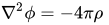
${\displaystyle \nabla ^{2}\phi =-4\pi \rho \;}$

today named after him Poisson's equation or the potential theory equation, was first published in the Bulletin de la société philomatique (1813). If ρ = 0, we get Laplace's equation:

${\displaystyle \nabla ^{2}\phi =0\;.}$

In 1812 Poisson discovered that Laplace's equation is valid only outside of a solid. A rigorous proof for masses with variable density was first given by Carl Friedrich Gauss in 1839. Both equations have their equivalents in vector algebra. Poisson's equation for the divergence of the gradient of a scalar field, φ in 3-dimensional space is:

${\displaystyle \nabla ^{2}\phi =\rho (x,y,z)\;.}$

Consider for instance Poisson's equation for surface electrical potential, Ψ as a function of the density of electric charge, ρ_e at a particular point:

${\displaystyle \nabla ^{2}\Psi ={\partial ^{2}\Psi \over \partial x^{2}}+{\partial ^{2}\Psi \over \partial y^{2}}+{\partial ^{2}\Psi \over \partial z^{2}}=-{\rho _{e} \over \varepsilon \varepsilon _{0}}\;.}$

The distribution of a charge in a fluid is unknown and we have to use the Poisson–Boltzmann equation:

${\displaystyle \nabla ^{2}\Psi ={n_{0}e \over \varepsilon \varepsilon _{0}}\left(e^{e\Psi (x,y,z)/k_{B}T}-e^{-e\Psi (x,y,z)/k_{B}T}\right),\;}$

which in most cases cannot be solved analytically. In polar coordinates the Poisson–Boltzmann equation is:

${\displaystyle {1 \over r^{2}}{d \over dr}\left(r^{2}{d\Psi \over dr}\right)={n_{0}e \over \varepsilon \varepsilon _{0}}\left(e^{e\Psi (r)/k_{B}T}-e^{-e\Psi (r)/k_{B}T}\right)\;}$

which also cannot be solved analytically. If a field, φ is not scalar, the Poisson equation is valid, as can be for example in 4-dimensional Minkowski space:

${\displaystyle {\sqrt {\phi }}_{ik}=\rho (x,y,z,ct)\;.}$

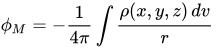
If ρ(x, y, z) is a continuous function and if for r→ ∞ (or if a point 'moves' to infinity) a function φ goes to 0 fast enough, a solution of Poisson's equation is the Newtonian potential of a function ρ(x, y, z):

${\displaystyle \phi _{M}=-{1 \over 4\pi }\int {\rho (x,y,z)\,dv \over r}\;}$

where r is a distance between a volume element dv and a point M. The integration runs over the whole space.
Another "Poisson's integral" is the solution for the Green function for Laplace's equation with Dirichlet condition over a circular disk:

${\displaystyle \phi (\xi \eta )={1 \over 4\pi }\int _{0}^{2\pi }{R^{2}-\rho ^{2} \over R^{2}+\rho ^{2}-2R\rho \cos(\psi -\chi )}\phi (\chi )\,d\chi \;}$

where

${\displaystyle \xi =\rho \cos \psi ,\;}$

${\displaystyle \quad \eta =\rho \sin \psi ,\;}$

φ is a boundary condition holding on the disk's boundary.

In the same manner, we define the Green function for the Laplace equation with Dirichlet condition, ∇² φ = 0 over a sphere of radius R. This time the Green function is:

${\displaystyle G(x,y,z;\xi ,\eta ,\zeta )={1 \over r}-{R \over r_{1}\rho }\;,}$

where

${\displaystyle \rho ={\sqrt {\xi ^{2}+\eta ^{2}+\zeta ^{2}}}}$ is the distance of a point (ξ, η, ζ) from the center of a sphere,

r is the distance between points (x, y, z) and (ξ, η, ζ), and
r₁ is the distance between the point (x, y, z) and the point (Rξ/ρ, Rη/ρ, Rζ/ρ), symmetrical to the point (ξ, η, ζ).
Poisson's integral now has a form:

${\displaystyle \phi (\xi ,\eta ,\zeta )={1 \over 4\pi }\iint _{S}{R^{2}-\rho ^{2} \over Rr^{3}}\phi \,ds\;.}$

Poisson's two most important memoirs on the subject are Sur l'attraction des sphéroides (Connaiss. ft. temps, 1829), and Sur l'attraction d'un ellipsoide homogène (Mim. ft. l'acad., 1835). In concluding our selection from his physical memoirs, we may mention his memoir on the theory of waves (Mém. ft. l'acad., 1825).
In pure mathematics, his most important works were his series of memoirs on definite integrals and his discussion of Fourier series, the latter paving the way for the classic researches of Peter Gustav Lejeune Dirichlet and Bernhard Riemann on the same subject; these are to be found in the Journal of the École Polytechnique from 1813 to 1823, and in the Memoirs de l'Académie for 1823. He also studied Fourier integrals. We may also mention his essay on the calculus of variations (Mem. de l'acad., 1833), and his memoirs on the probability of the mean results of observations (Connaiss. d. temps, 1827, &c). The Poisson distribution in probability theory is named after him.
In his Traité de mécanique (2 vols. 8vo, 1811 and 1833), which was written in the style of Laplace and Lagrange and was long a standard work, he showed many novelties such as an explicit usage of momenta:

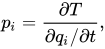
${\displaystyle p_{i}={\partial T \over {\partial q_{i}/\partial t}},}$

which influenced the work of Hamilton and Jacobi.
(7)
Jules Henri Poincaré (French: [ʒyl ɑ̃ʁi pwɛ̃kaʁe];^[2][3] 29 April 1854 – 17 July 1912) was a French mathematician, theoretical physicist, engineer, and philosopher of science. He is often described as a polymath, and in mathematics as The Last Universalist by Eric Temple Bell,^[4] since he excelled in all fields of the discipline as it existed during his lifetime.
As a mathematician and physicist, he made many original fundamental contributions to pure and applied mathematics, mathematical physics, and celestial mechanics.^[5] He was responsible for formulating the Poincaré conjecture, which was one of the most famous unsolved problems in mathematics until it was solved in 2002–2003. In his research on the three-body problem, Poincaré became the first person to discover a chaotic deterministic system which laid the foundations of modern chaos theory. He is also considered to be one of the founders of the field of topology.
(8) Sir Andrew John Wiles KBE FRS (born 11 April 1953^[1]) is a British mathematician and a Royal Society Research Professor at the University of Oxford, specialising in number theory. He is most notable for proving Fermat's Last Theorem, for which he received the 2016 Abel Prize.^[4][5][6] Wiles has received numerous other honours.
(9)
Nikolai Ivanovich Lobachevsky (Russian: Никола́й Ива́нович Лобаче́вский; IPA: [nʲikɐˈlaj ɪˈvanəvʲɪtɕ ləbɐˈtɕɛfskʲɪj] 1 December [O.S. 20 November] 1792 – 24 February [O.S. 12 February] 1856) was a Russian mathematician and geometer, known primarily for his work on hyperbolic geometry, otherwise known as Lobachevskian geometry.
William Kingdon Clifford called Lobachevsky the "Copernicus of Geometry" due to the revolutionary character of his work.
(10) Augustus De Morgan (/dɪ ˈmɔːrɡən/;^[1] 27 June 1806 – 18 March 1871) was a British mathematician and logician. He formulated De Morgan's laws and introduced the term mathematical induction, making its idea rigorous.

De Morgan was a brilliant and witty writer, whether as a controversialist or as a correspondent. In his time there flourished two Sir William Hamiltons who have often been conflated. One was Sir William Hamilton, 9th Baronet (that is, his title was inherited), a Scotsman, professor of logic and metaphysics at the University of Edinburgh; the other was a knight (that is, won the title), an Irishman, professor at astronomy in the University of Dublin. The baronet contributed to logic, especially the doctrine of the quantification of the predicate; the knight, whose full name was William Rowan Hamilton, contributed to mathematics, especially geometric algebra, and first described the Quaternions. De Morgan was interested in the work of both, and corresponded with both; but the correspondence with the Scotsman ended in a public controversy, whereas that with the Irishman was marked by friendship and terminated only by death. In one of his letters to Rowan, De Morgan says,

Be it known unto you that I have discovered that you and the other Sir W. H. are reciprocal polars with respect to me (intellectually and morally, for the Scottish baronet is a polar bear, and you, I was going to say, are a polar gentleman). When I send a bit of investigation to Edinburgh, the W. H. of that ilk says I took it from him. When I send you one, you take it from me, generalize it at a glance, bestow it thus generalized upon society at large, and make me the second discoverer of a known theorem.

The correspondence of De Morgan with Hamilton the mathematician extended over twenty-four years; it contains discussions not only of mathematical matters, but also of subjects of general interest. It is marked by geniality on the part of Hamilton and by wit on the part of De Morgan.

Denotation and Connotation

• Denotation refers to the literal meaning of a word, the "dictionary definition."¨ For example, if you look up the word snake in a dictionary, you will discover that one of its denotative meanings is "any of numerous scaly, legless, sometimes venomous reptiles¡Khaving a long, tapering, cylindrical body and found in most tropical and temperate regions."
• Connotation, on the other hand, refers to the associations that are connected to a certain word or the emotional suggestions related to that word. The connotative meanings of a word exist together with the denotative meanings. The connotations for the word snake could include evil or danger.

 

• Denotation refers to the literal meaning of a word, the "dictionary definition."¨ For example, if you look up the word snake in a dictionary, you will discover that one of its denotative meanings is "any of numerous scaly, legless, sometimes venomous reptiles¡Khaving a long, tapering, cylindrical body and found in most tropical and temperate regions."
• Connotation, on the other hand, refers to the associations that are connected to a certain word or the emotional suggestions related to that word. The connotative meanings of a word exist together with the denotative meanings. The connotations for the word snake could include evil or danger.

English -by:Rea Ylanan

The Real Number System

The real number system evolved over time by expanding the notion of what we mean by the word “number.” At first, “number” meant something you could count, like how many sheep a farmer owns. These are called the natural numbers, or sometimes the counting numbers.

Natural Numbers

or “Counting Numbers”

1, 2, 3, 4, 5, . . .

• The use of three dots at the end of the list is a common mathematical notation to indicate that the list keeps going forever.

At some point, the idea of “zero” came to be considered as a number. If the farmer does not have any sheep, then the number of sheep that the farmer owns is zero. We call the set of natural numbers plus the number zero the whole numbers.

Whole Numbers

Natural Numbers together with “zero”

0, 1, 2, 3, 4, 5, . . .

About the Number Zero What is zero? Is it a number? How can the number of nothing be a number? Is zero nothing, or is it something? Well, before this starts to sound like a Zen koan, let’s look at how we use the numeral “0.” Arab and Indian scholars were the first to use zero to develop the place-value number system that we use today. When we write a number, we use only the ten numerals 0, 1, 2, 3, 4, 5, 6, 7, 8, and 9. These numerals can stand for ones, tens, hundreds, or whatever depending on their position in the number. In order for this to work, we have to have a way to mark an empty place in a number, or the place values won’t come out right. This is what the numeral “0” does. Think of it as an empty container, signifying that that place is empty. For example, the number 302 has 3 hundreds, no tens, and 2 ones. So is zero a number? Well, that is a matter of definition, but in mathematics we tend to call it a duck if it acts like a duck, or at least if it’s behavior is mostly duck-like. The number zero obeys most of the same rules of arithmetic that ordinary numbers do, so we call it a number. It is a rather special number, though, because it doesn’t quite obey all the same laws as other numbers—you can’t divide by zero, for example. Note for math purists: In the strict axiomatic field development of the real numbers, both 0 and 1 are singled out for special treatment. Zero is the additive identity, because adding zero to a number does not change the number. Similarly, 1 is the multiplicative identity because multiplying a number by 1 does not change it.

Even more abstract than zero is the idea of negative numbers. If, in addition to not having any sheep, the farmer owes someone 3 sheep, you could say that the number of sheep that the farmer owns is negative 3. It took longer for the idea of negative numbers to be accepted, but eventually they came to be seen as something we could call “numbers.” The expanded set of numbers that we get by including negative versions of the counting numbers is called the integers.

Integers

Whole numbers plus negatives

. . . –4, –3, –2, –1, 0, 1, 2, 3, 4, . . .

About Negative Numbers How can you have less than zero? Well, do you have a checking account? Having less than zero means that you have to add some to it just to get it up to zero. And if you take more out of it, it will be even further less than zero, meaning that you will have to add even more just to get it up to zero. The strict mathematical definition goes something like this: For every real number n, there exists its opposite, denoted – n, such that the sum of n and – n is zero, or n + (– n) = 0 Note that the negative sign in front of a number is part of the symbol for that number: The symbol “–3” is one object—it stands for “negative three,” the name of the number that is three units less than zero. The number zero is its own opposite, and zero is considered to be neither negative nor positive. Read the discussion of subtraction for more about the meanings of the symbol “–.”

The next generalization that we can make is to include the idea of fractions. While it is unlikely that a farmer owns a fractional number of sheep, many other things in real life are measured in fractions, like a half-cup of sugar. If we add fractions to the set of integers, we get the set of rational numbers.

Rational Numbers

All numbers of the form , where a and b are integers (but b cannot be zero)
Rational numbers include what we usually call fractions

• Notice that the word “rational” contains the word “ratio,” which should remind you of fractions.

The bottom of the fraction is called the denominator. Think of it as the denomination—it tells you what size fraction we are talking about: fourths, fifths, etc.

The top of the fraction is called the numerator. It tells you how many fourths, fifths, or whatever.

• RESTRICTION: The denominator cannot be zero! (But the numerator can)

If the numerator is zero, then the whole fraction is just equal to zero. If I have zero thirds or zero fourths, than I don’t have anything. However, it makes no sense at all to talk about a fraction measured in “zeroths.”

• Fractions can be numbers smaller than 1, like 1/2 or 3/4 (called proper fractions), or they can be numbers bigger than 1 (called improper fractions), like two-and-a-half, which we could also write as 5/2

All integers can also be thought of as rational numbers, with a denominator of 1:

This means that all the previous sets of numbers (natural numbers, whole numbers, and integers) are subsets of the rational numbers.
Now it might seem as though the set of rational numbers would cover every possible case, but that is not so. There are numbers that cannot be expressed as a fraction, and these numbers are called irrational because they are not rational.

Irrational Numbers

• Cannot be expressed as a ratio of integers.
• As decimals they never repeat or terminate (rationals always do one or the other)

Examples: 

	Rational (terminates)
	Rational (repeats)
	Rational (repeats)
	Rational (repeats)
	Irrational (never repeats or terminates)
	Irrational (never repeats or terminates)

 

More on Irrational Numbers It might seem that the rational numbers would cover any possible number. After all, if I measure a length with a ruler, it is going to come out to some fraction—maybe 2 and 3/4 inches. Suppose I then measure it with more precision. I will get something like 2 and 5/8 inches, or maybe 2 and 23/32 inches. It seems that however close I look it is going to be some fraction. However, this is not always the case. Imagine a line segment exactly one unit long: Now draw another line one unit long, perpendicular to the first one, like this: Now draw the diagonal connecting the two ends: Congratulations! You have just drawn a length that cannot be measured by any rational number. According to the Pythagorean Theorem, the length of this diagonal is the square root of 2; that is, the number which when multiplied by itself gives 2. According to my calculator, But my calculator only stops at eleven decimal places because it can hold no more. This number actually goes on forever past the decimal point, without the pattern ever terminating or repeating. This is because if the pattern ever stopped or repeated, you could write the number as a fraction—and it can be proven that the square root of 2 can never be written as for any choice of integers for a and b. The proof of this was considered quite shocking when it was first demonstrated by the followers of Pythagoras 26 centuries ago.

The Real Numbers

• Rationals + Irrationals
• All points on the number line
• Or all possible distances on the number line

When we put the irrational numbers together with the rational numbers, we finally have the complete set of real numbers. Any number that represents an amount of something, such as a weight, a volume, or the distance between two points, will always be a real number. The following diagram illustrates the relationships of the sets that make up the real numbers.

An Ordered Set

The real numbers have the property that they are ordered, which means that given any two different numbers we can always say that one is greater or less than the other. A more formal way of saying this is:
For any two real numbers a and b, one and only one of the following three statements is true:

1.      a is less than b, (expressed as a < b)

2.      a is equal to b, (expressed as a = b)

3.      a is greater than b, (expressed as a > b)

The Number Line

The ordered nature of the real numbers lets us arrange them along a line (imagine that the line is made up of an infinite number of points all packed so closely together that they form a solid line). The points are ordered so that points to the right are greater than points to the left:

• Every real number corresponds to a distance on the number line, starting at the center (zero).
• Negative numbers represent distances to the left of zero, and positive numbers are distances to the right.
• The arrows on the end indicate that it keeps going forever in both directions.

Absolute Value 

When we want to talk about how “large” a number is without regard as to whether it is positive or negative, we use the absolute value function. The absolute value of a number is the distance from that number to the origin (zero) on the number line. That distance is always given as a non-negative number.
In short:

• If a number is positive (or zero), the absolute value function does nothing to it:
• If a number is negative, the absolute value function makes it positive:

WARNING: If there is arithmetic to do inside the absolute value sign, you must do it before taking the absolute value—the absolute value function acts on the result of whatever is inside it. For example, a common error is

   (WRONG)

The correct result is

Axioms, Properties and Definitions of Real Numbers

Axioms, Properties and Definitions of Real Numbers

 

 

Definitions

 

1.Property of a number system–a fact that is true regarding that system

 

2.Axiom–a property that forms the framework for the system. It does not require any proof. We assume that it is true.

 

   3.Term–a combination of numbers and variables that are multiplied together.

 

4.Like terms–two or more terms that have the identical variables raised to the same power(s).

 

 5.Coefficient–the number multiplying a variable in a term.If there is no written number, it is assumed to be 1.

 

  6.Expression–a combination of terms added together

 

7.Equation–A combination of terms added together that contains an equal sign

 

  8.Inequality–A combination of terms added together that contains an greater than, less than, greater than or equal to, less than or equal  to.

 

9.Factor–a combination of numbers and variables that divides into a term evenly.

 

10.Common Factor–a combination of numbers and variables that is a factor of each in an expression

Field Axioms/Properties (1)

Properties of Real Numbers

The following table lists the defining properties of the real numbers (technically called the field axioms). These laws define how the things we call numbers should behave.

Addition	Multiplication
Commutative For all real a, b a + b = b + a	Commutative For all real a, b ab = ba
Associative For all real a, b, c a + (b + c) = (a + b) + c	Associative For all real a, b, c (ab)c = a(bc)
Identity There exists a real number 0 such that for every real a a + 0 = a	Identity There exists a real number 1 such that for every real a a × 1 = a
Additive Inverse (Opposite) For every real number a there exist a real number, denoted (-a), such that a + (–a) = 0	Multiplicative Inverse (Reciprocal) For every real number a except 0 there exist a real number, denoted , such that a ×  = 1
Distributive Law For all real a, b, c a(b + c) = ab + ac, and (a + b)c = ac + bc

The commutative and associative laws do not hold for subtraction or division:

a – b is not equal to b – a

a ÷ b is not equal to b ÷ a

a – (b – c) is not equal to (a – b) – c

a ÷ (b ÷ c) is not equal to (a ÷ b) ÷ c

Try some examples with numbers and you will see that they do not work.

What these laws mean is that order and grouping don't matter for addition and multiplication, but they certainly do matter for subtraction and division. In this way, addition and multiplication are “cleaner” than subtraction and division. This will become important when we start talking about algebraic expressions. Often what we will want to do with an algebraic expression will involve rearranging it somehow. If the operations are all addition and multiplication, we don't have to worry so much that we might be changing the value of an expression by rearranging its terms or factors. Fortunately, we can always think of subtraction as an addition problem (adding the opposite), and we can always think of division as a multiplication (multiplying by the reciprocal).
You may have noticed that the commutative and associative laws read exactly the same way for addition and multiplication, as if there was no difference between them other than notation. The law that makes them behave differently is the distributive law, because multiplication distributes over addition, not vice-versa.. The distributive law is extremely important, and it is impossible to understand algebra without being thoroughly familiar with this law.
Example:  2(3 + 4)
According to the order of operations rules, we should evaluate this expression by first doing the addition inside the parentheses, giving us

2(3 + 4) = 2(7) = 14

But we can also look at this problem with the distributive law, and of course still get the same answer. The distributive law says that